
Blog


Optimizing Color Data in FRED
Introduction
In many real-world applications of products containing illumination systems, it is important to predict or specify the output colour(s) of the system. FRED can evaluate and optimize spectral power data in order to give the desired CIE chromaticity coordinates. This article will discuss using FRED’s optimizer to alter tristimulus values and target a desired color using chromaticity coordinates, as well as highlighting the Color Image calculation capabilities.
LED Spectrum Using Digitizer
To attain the most accurate recreation of the LED sources, we first start by creating our red, green and blue color spectra. A simple way to do this quickly is to take advantage of FRED’s digitizer function. The Digitization Tool (or Digitizer) allows the user to digitize data points from a graph, plot, lens drawing, etc. from an image file. This can be accessed in FRED when creating a new Sampled spectrum and then selecting Digitize Curve.
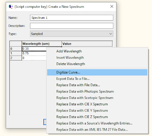
From here we are then able to select an image of a spectrum and insert it into our digitizer. It is important to note that FRED’s default units are microns along the x axis and watts along the y axis.
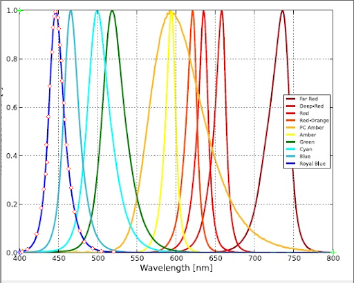
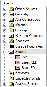
After setting the min X and Y values to be at the origin (0.4,0). We then set our max X value to be 0.8 microns and the max Y value to be 1 Watt. Next, we select the data points along our desired curve and finally select export data (You also have the option to save the digitized data to file so you can use the digitized data elsewhere). After exporting the data, the spectra for each LED can be seen in the Spectra folder.
Display
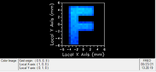
For this demonstration, we use a simple RGB LED system to under light a single F key on a computer keyboard.
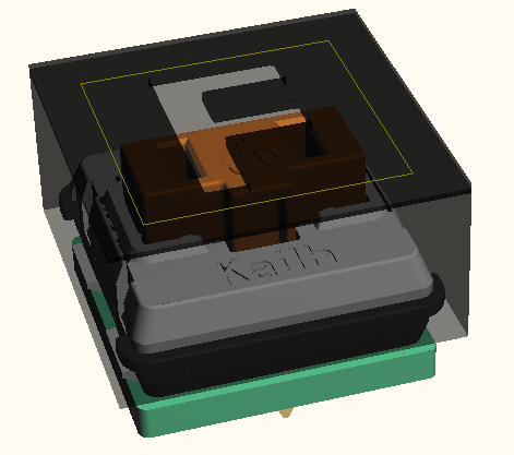
The LED source is projected into free space and scattered underneath the key cover. The light then exits through the opening on the top thus illuminating the letter and stopping on our analysis surface.
Following the raytrace we can view the color of the illumination with the Color Image analysis feature.
Color Image
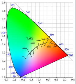
The Color Image analysis feature calculates the XYZ chromaticity coordinates (CIE 1931) for each pixel of the selected analysis surface and then converts the chromaticity coordinates to RGB values for display in the Chart Viewer. FRED performs this analysis by:
1/ Determining the maximum Y tristimulus value in the dataset
2/ Scale each tristimulus value by the factor: brightness/Ymax
3/ Convert from scaled XYZ tristimulus to RGB using the sRGB matrix:
[ 3.2406 -1.5372. -0.4986 ]
[-0.9689 1.8758. 0.0415 ]
[ 0.0557 -0.2040 1.0570 ]
4/ R,G,B values outside of the range from 0 to 1.0 are considered "out of gamut" and clamped at either 0 or 1.0
5/ Apply gamma correction (gamma = 2.2) to the RGB pixel values (ex. R = R1 / 2.2)
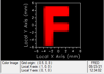
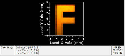
The Color Image chart view has four panes; an RGB spatial map on the analysis surface, two cross-sectional profiles, and a chromaticity diagram. As the cursor is moved in the spatial map a cursor in the chromaticity diagram indicates the XY chromaticity coordinate corresponding to the current pixel. Thus with our previously defined Spectral data we obtain the following color image:
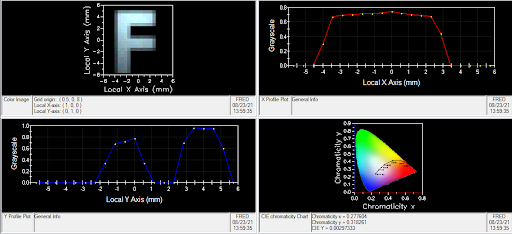
Not only are we able to view the color image in the top left, but also the chromaticity X and Y values pertaining to each pixel in the bottom right. Here we see the key color appears to be white(ish) when all three LEDs have equal power.
Optimization and Merit Aberrations Functions
To obtain a desired color output, FRED uses the optimizer to tune the relative powers of the three LEDs, producing a new color, and illuminating the computer key.
The red, green and blue LEDs are selected as entities and assigned the “Source power” Type.
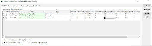
This lets the optimizer know which model parameters are to be varied during the optimization. The upper and lower limits correspond to the type selected. For Source power, the upper and lower limits pertain to the power in watts for each LED source.
The optimizer’s Merit Function Aberrations are the individual components from which the merit function is constructed. Each aberration defines the quantity to be evaluated (ex. spot size, total power), a weighting factor,and the desired target value to be achieved. All active aberrations are summed into the merit function in the following way:
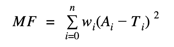
Where wi is the weighting factor for the i'th aberration, Ai is the computed quantity for the i'th aberration and Ti is the target value for the i'th aberration.
The Merit Function Aberrations tab is where we select our Aberration Definition as well as the analysis surface that will be used to calculate the merit function.
The ‘Centroid X color’ and ‘Centroid Y color’ are used for the Aberration Definitions, with targeted chromaticity values corresponding to our desired color on the chromaticity diagram. This calculates the x,y chromaticity coordinates for each pixel in the analysis grid. The flux-weighted average x chromaticity or y chromaticity value in the data grid is returned as the aberration value.
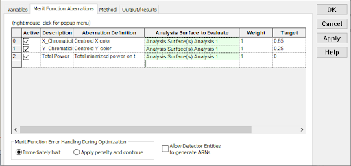
The values chosen above give us chromaticity coordinates in the red spectrum.
The Method tab is used to define the optimization method as well as the number of iterations. When altering power values, the Simplex method (Geometric approach) can be used with a maximum of 20 iterations.
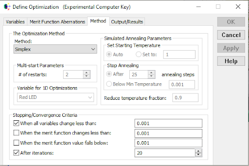
By applying “When all variables change less than:” we allow FRED to speed up the convergence process by stopping the optimization when arriving at our desired values. Depending on the required change in values, we may need more than 20 iterations, however; small changes will converge in less than 20 iterations.
The Output/Results tab allows for the selection of how the optimization status and results are conveyed back to the user. Rays can be drawn to the screen and the 3D view updated during optimization, and the merit function and variable values can be printed to the output window in text format. Here we are asking FRED to print the merit function for each iteration and to print the previous and current values after optimization. This way we can ensure our spectral power values have been optimized.
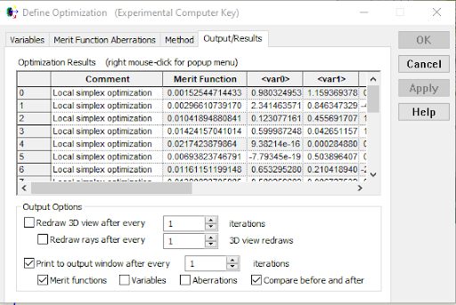
After selecting to run the Optimizer, FRED will immediately display all selected criteria in the output window and begin displaying merit function values for each iteration.
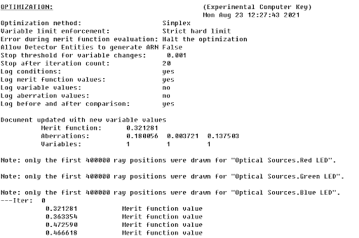
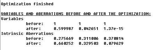
After FRED is done running all the iterations, “Optimization finished” will appear in the output window and below will be the variables and aberrations before and after optimization. The variables are placed in order from right to left displaying red, green and blue power values.
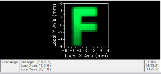
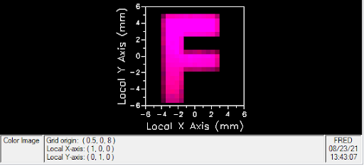
We are now able to view our new color image.
Color Diagrams
Now that we have defined our tristimulus values and optimized the system, we go back to the Color Image Object.
As expected from our centroid x and y values, we see the letter F printed in red. When looking at the output window it can be seen that our red LED has been optimized to produce the most power and that our green and blue LEDs have been largely reduced, thus, giving us a red spectrum. To better see FREDs ability to optimize the spectral power of our three sources, We run the optimizer for a variety of CIE chromaticity values.

Centroid X Color = 0.2, Centroid Y Color = 0.1
LED Power (Watts)
Red = 0.0986, Green = 0.157, Blue = 0.709
Centroid X Color = 0.1, Centroid Y Color = 0.7
LED Power (Watts)
Red = 0.0765, Green = 0.678, Blue = 0.0231
Centroid X Color = 0.55, Centroid Y Color = 0.4
LED Power (Watts)
Red = 0.0642, Green = 0.0211, Blue = 0.0
Centroid X Color = 0.45, Centroid Y Color = 0.15
LED Power (Watts)
Red = 0.199, Green = 0.0105, Blue = 0.0914
FRED is able to alter the spectral power of our RGB LED system to obtain all colors on the visible light spectrum. Contact us to request a Demo of FRED or talk through your application needs in more detail.