
Blog


Time of Flight Simulations in FRED
Time of flight (ToF) sensing is a key technology in advanced driver-assistance systems (ADAS) such as LiDAR, and can also be found on consumer electronic devices such as phones. The specifics of the optical set-ups may vary depending on the application but the principles are the same - detection of distance by measuring the time it takes for light to make a round trip from a source to an object and scatter back to a detector.
Although optical software is generally restricted to the spatial domain, a time of flight calculation can be constructed from the optical path length that rays travel. In the following examples we will demonstrate how FRED can be used to simulate this. Our first example is a fun ToF measurement of the distance of chess pieces on a board, our second example is of Automotive LiDAR.
Chess Board Example
First, we’ll take a simple set-up consisting of a source (emitting uniformly into an angle), a chess board as an object to interact with and determine distance, and an imaging system comprising an ideal lens focusing the scattered light onto an analysis surface combined with a detector.

After tracing 500,000 rays (not shown above) and capturing the back scattered light the Irradiance captured on the detector is shown below:

In this example the chess board and pieces have a higher degree of backscatter than the box they are placed inside which is why their irradiance is higher. This is not a requirement, it simply makes the Irradiance map more interesting to look at for our example.
To extract the ToF data FRED’s simple but powerful scripting capability is used. The script filters the ray set captured on the analysis surface to the shortest optical path length (OPL) and creates an Analysis Result Node (ARN) for the irradiance at that distance - it then loops over the ray set from the initial closest object to the most distant - refiltering the OPL range of interest and creating an ARN for each step. Having created an ARN for each OPL range these results are then looped over in a second pass to extract the power values at each distance/time step and chart out the following items of interest.
ToF (Irradiance vs Time)

Note the X-axis is time in nanoseconds. The peaks in backscattered light correspond to the objects in the scene.
Distance Map

Note that the false colour scale is distance in millimeters.
ToF Irradiance Movie

FRED also allows us to easily combine a set of ARNs into a movie, thus allowing us to view the time evolution of the Irradiance on the detector. As we step through the frames recorded by our detector we can see the objects our source is scattering back from.
LiDAR Example
The same methodology can be applied to more complex scenes at larger scales such as automotive LiDAR. In this example a street scene has been built in FRED using imported CAD objects.

In just a few minutes of processing a larger set of 10 million rays we can generate the scene irradiance and extract distance information from our dataset.
Scene Irradiance

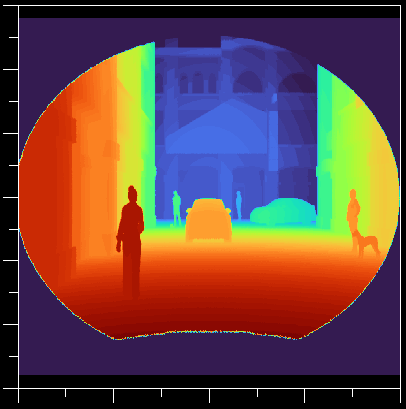
Distance Map

Note how the distance map teases out the detail in the building at the end of the street, including the person standing in the far distance between the two cars. For reference the deep red corresponds to a distance of ~5m, indigo represents ~32m and the colour steps represent approximately 30cm resolution.
Summary
FRED’s powerful raytrace engine, analysis tools and scripting offers everything that is needed to simulate your Time of Flight systems. Contact us to request a Demo of FRED or talk through your application needs in more detail.
Tags: